Part 2 – Non-linear analysis

Each time we’re facing a non-linearity in a model (either mechanical or geometric) we need a non-linear analysis. Mainly, they can be categorized in static and dynamic analyses:

- In static analysis, the system of equations to be solved is  , where K is the stiffness matrix, u the vector collecting the nodal displacements and rotations and F the applied force vector. In this kind of analysis, the time variable is used only to order results (t=0.1 precedes t=0.15, etc.), hence velocities and accelerations are always zero.

- In dynamic analysis, the system of equation to be solved is , which involves the mass matrix , the stiffness matrix and the damping matrix . is the displacement vector we want to find as solution of the system,  is the dragging vector, which specifies for which spatial directions the external ground acceleration  is applied.

It’s time to introduce the concept of second-order effects. The simplest second-order effect to be considered on beam is the so-called P-Delta effect. Let’s take a simple cantilever column with a lateral and a compression load. Once the lateral load is applied, the vertical loading on top cause an additional second-order moment if the equilibrium is computed on deformed shape.

A geometric stiffness matrix Kg is computed every time the user asks for second-order effects – such matrix is a function of the applied loading condition. Hence, a PDelta analysis search iteratively the equilibrium considering both K and Kg. The same occurs if user selects “2^nd order” option in a non-linear analysis, with the main difference that the second-order effects in this case are fully considered for all the supported elements in the model.

The most common NL analyses are static and dynamic, with or without second-order effects. The most used static NL analysis is the so-called pushover, in which a building model is pushed in a chosen direction by a set of forces for each storey. The shape of the force vectors is called distribution, typically plotted over height. We can distinguish two main distributions, that represent the upper and lower limit of the pushover curves:

- Modal or inverse-triangular distribution, in which lateral forces increase with building height. This distribution typically minimize the total base shear and maximize ductility of the structure;

- Uniform distribution, proportional to masses if all storey are equally loaded. This distribution typically maximize the total base shear and minimize ductility of the structure.

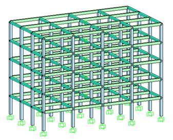
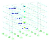
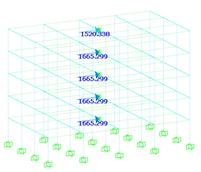
RC building as case study (left) and storey forces distributions (right)

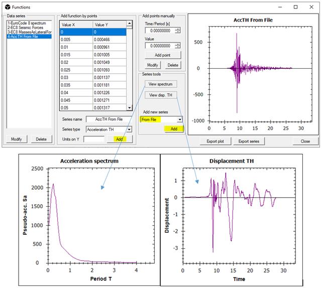
To obtain the storey forces for pushover, there are special built-in functions in NextFEM Designer. In Edit / Functions… window, you can find these commands to generate new series:

- EC8 Seismic Forces, that generates an inverse-triangular distribution for the building. You have to refer to a previously added seismic spectrum function, and model must have rigid diaphragms. Lateral forces are automatically assigned to the selected loadcases;

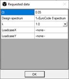
- EC8 Masses as Lateral Forces, which generated a uniform-like lateral forces distribution. Again, rigid diaphragms are required in order to proceed.

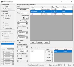
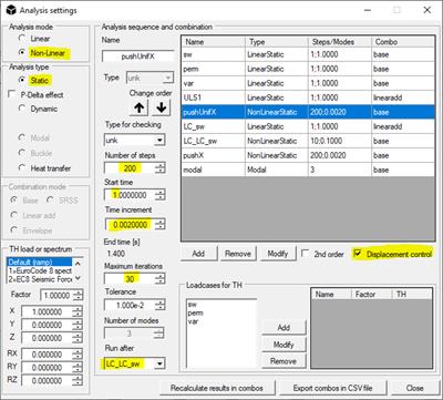
For pushover analyses, it is a good practice to proceed in displacement control by activating the proper option in Assign / Analysis settings: this means that our analysis will be guided by the displacement of a chosen node, usually taken on the barycentre of the roof. Such setting permits to the NL analysis to go through the strength losses that can occur during pushover, for example when a hinge reaches failure. We call this “control node”.

In addition, it is of fundamental importance to set the following properties of non-linear static analysis:

- Adequate number of steps: the load will be applied incrementally, and each increment is equal to final load / number of steps;

- The start time is automatically adapted if Run after is not empty. A pushover analysis must be conducted after the vertical loads are applied;

- Displacement control option is enabled. The barycentric node of roof is automatically suggested. Users have to specify the push-over direction;

- Time increment has to be set as a small amount. Total load and final load can be different, since the analysis terminated when all required steps have been performed, hence final load = steps * time increment. In static analysis, time is assumed as proportional with load. In case of a sequence of analysis, the proportionality starts at the end of preceding analysis (vertical loading goes from t=0 to t=1, subsequent pushover starts from t=1).

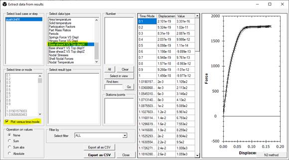
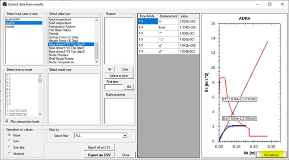
Some post processing tools are available in Extract data window, including the global pushover curve check conducted with the N2 method. This feature is freely accessible without any license, as well as fiber models.

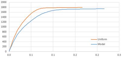
Pushover curves of a fiber model of RC frame with uniform and modal distributions

Dynamic non-linear analysis requires masses in the model. In NextFEM Designer, masses are assigned automatically from load cases (load to mass, including self-weight) or can be set manually for each node. In any case, only nodal masses are handled.

Dynamic analysis has been implemented to work with applied ground motions, applied uniformly to all the restrained nodes (typically the base nodes). A ground motion is represented by an acceleration time-history: in the default solver, this is automatically converted to a displacement time history and applied to the bounded nodes; in OpenSees, an acceleration timeSeries is applied. All model functions can be set in Assign / Functions. If loaded from file, a 2 column time vs. acceleration format is required. Use dot as decimal separator.

Units in gal (cm/s^2)

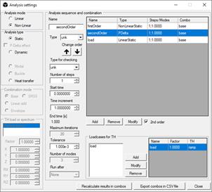
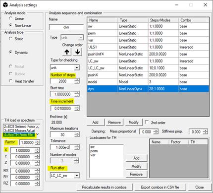
The non-linear dynamic analysis can be set as follows. It is important to select:

- The proper Time-History (TH) in the TH load or spectrum box and its factors: Factor is a global factor, while parameters X,Y,Z,RX,RY,RZ determine the direction of ground motion;

- When TH is selected, the number of steps is automatically updated with total duration. Increase the number of steps and set a proper time increment, as to maintain the same total time;

- Using built-in solver with a sequence of analyses, a dynamic analysis must be preceded by an analysis of the same type. Typically, user can set a dynamic analysis with a large damping. OpenSees solver accepts a static analysis preceding the dynamic, as in the following picture;

- The proper damping, which can be set as per the Rayleigh proportional damping model. The damping matrix is set through a mass proportional term  and a stiffness proportional :

In which  is the critical damping ratio and T is the period of interest, usually the fundamental one if its mass participation is enough to be representative.

Please note that results from the built-in solver can be stored even from an unfinished non-linear analysis (Tools / Options / Write temporary results must be unchecked), while from OpenSees solver this would not happen.